Waterfall charts can look a bit complicated if you've never used one before. They've got floating bars, stacked values, and a style that feels more advanced than your typical bar or column chart. But once you understand how they work, they become one of the easiest ways to explain how a number changes over time or across different factors. Whether you're laying out a financial report, analyzing performance metrics, or breaking down steps in a budget, this type of chart helps make the numbers easier to follow.

If you’re using Excel 2016 or later, you already have the tool built in—no need for templates or add-ons.

What a Waterfall Chart Shows

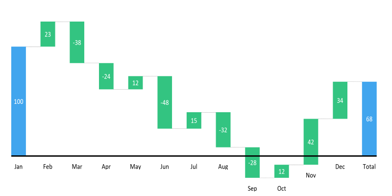
This chart works by displaying a starting point, followed by a series of increases and decreases, and ending with a final value. Each bar shows how much each factor contributes to that overall shift, whether it's a gain or a loss. Unlike a stacked column chart, which piles all the values together, a waterfall chart keeps each step clear. The bars "float" up or down depending on the value, and the total bars sit directly on the axis. This makes it easy to track what's helping or hurting your total—without scanning a spreadsheet full of raw numbers.

Step-by-Step: Building a Waterfall Chart in Excel

The process is more straightforward than most expect. Once your data is organized, it takes just a few clicks.

Step 1: Set Up the Data

Start by arranging the data in three simple columns:

• Category: Name of each step (like Starting Balance, Revenue, Expenses, etc.)
• Amount: Positive or negative numbers
• Type: Either “Total” or “Change”

Here’s a sample table:

This structure helps Excel identify which values are part of the running total and which ones stand on their own.

Step 2: Insert the Waterfall Chart

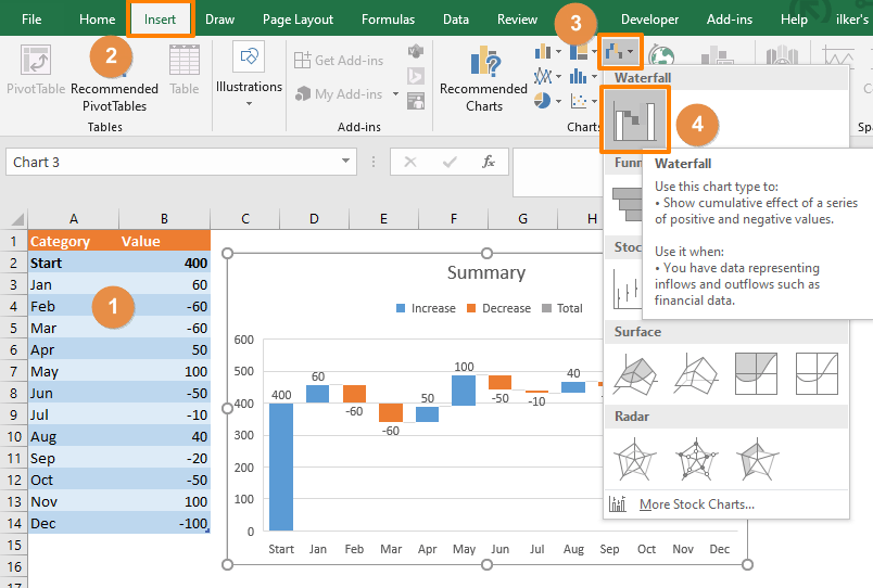
Once the data is in place:

1. Select all three columns in your table.
2. Go to the Insert tab in Excel’s ribbon.
3. In the Charts group, click on the Stock Chart button.
4. Select Waterfall.

At this point, Excel will generate a basic chart using the data you selected. Every bar will appear, but Excel might not recognize which ones are totals yet. That’s something you’ll adjust next.

Step 3: Mark Totals in the Chart

To make sure your chart correctly shows totals like the starting and ending values:

1. Click once on the chart.
2. Then, click again on a bar that represents a total (such as Starting Balance).
3. Right-click and select Set as Total.

Excel will shift the bar to anchor it directly on the horizontal axis. This tells Excel not to treat it as part of the cumulative series. Repeat this for any other total bars in your data, such as the Ending Balance.

Step 4: Tidy Up the Formatting

Now that the chart is showing the right structure, you can clean up the layout if you want a clearer or more polished look:

• To label the numbers, Click on the chart, then the + button in the top-right corner, and check Data Labels.
• To adjust colors, Click any bar, right-click, and go to Format Data Series to pick different fills for positive, negative, and total bars.
• To change or remove gridlines, axis labels, or the legend, Use the same + button to toggle what you want to keep or leave out.

You don’t have to do all of this, but if your chart is being shared with others or added to a presentation, it’s worth taking a minute to make it easier to read.

Custom Edits That Make a Difference

There are a few extra adjustments you can make to improve the chart’s readability, especially when the data range is wide or when the changes are small compared to the totals.

Adjusting the Vertical Axis

If some values are much larger than others, the smaller changes might look flat. You can fix this by manually adjusting the scale:

1. Right-click the vertical axis.
2. Select Format Axis.
3. Set custom minimum and maximum bounds to better fit your dataset.

This helps give all steps a more proportional appearance so no detail gets overlooked.

Rearranging the Category Order

Waterfall charts follow the order in which your data appears in the table. If you want the steps to appear differently—say, to match a process or narrative—just rearrange the rows in your table. The chart will adjust automatically.

Giving the Chart a Clear Title

Click the chart title placeholder and type in something that directly explains what’s being shown. A simple label like “2024 Year-End Profit Breakdown” helps make your chart easier to understand without needing extra explanation.

Where This Chart Works Best

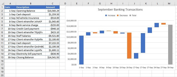
A waterfall chart is best used when there's a defined starting point, a final result, and a need to show how individual parts contributed to the change. That could be revenue shifts across departments, cost changes across a project timeline, or even things like how a product’s launch affected your monthly numbers.

It’s not the best choice for continuous trends or data with a lot of back-and-forth variation. But when you’re looking at specific step-by-step contributions to a change, it works better than most other chart types.

Done Right, It Explains Itself

After going through it once, the process becomes simple. What starts out looking technical becomes just another built-in feature of Excel you can use without a second thought. The real value is in how clearly the chart communicates the breakdown behind a number. Instead of just seeing that your result improved or declined, you can immediately understand why—and that's the kind of clarity that helps in both team meetings and reports.